The researchers identified two distinct events associated with Helene’s landfall. The first was its actual landfall along the Florida coast. The second was the intense rainfall on the North Carolina/Tennessee border. This rainfall came against a backdrop of previous heavy rain caused by a stalled cold front meeting moisture brought north by the fringes of the hurricane. These two regions were examined separately.
A changed climate
In these two regions, the influence of climate change is estimated to have caused a 10 percent increase in the intensity of the rainfall. That may not seem like much, but it adds up. Over both a two- and three-day window centered on the point of maximal rainfall, climate change is estimated to have increased rainfall along the Florida Coast by 40 percent. For the southern Appalachians, the boost in rainfall is estimated to have been 70 percent.
The probability of storms with the wind intensity of Helene hitting land near where it did is about a once-in-130-year event in the IRIS dataset. Climate change has altered that so it’s now expected to return about once every 50 years. The high sea surface temperatures that helped fuel Helene are estimated to have been made as much as 500 times more likely by our changed climate.
Overall, the researchers estimate that rain events like Helene’s landfall should now be expected about once every seven years, although the uncertainty is large (running from three to 25 years). For the Appalachian region, where rainfall events this severe don’t appear in our records, they are likely to now be a once-in-every-70-years event thanks to climate warming (with an uncertainty of between 20 and 3,000 years).
“Together, these findings show that climate change is enhancing conditions conducive to the most powerful hurricanes like Helene, with more intense rainfall totals and wind speeds,” the researchers behind the work conclude.
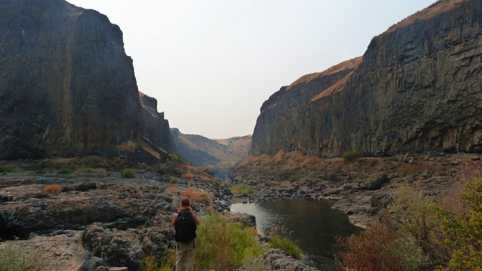
Enlarge/ Loads of lava: Kasbohm with a few solidified lava flows of the Columbia River Basalts.
Joshua Murray
As our climate warms beyond its historical range, scientists increasingly need to study climates deeper in the planet’s past to get information about our future. One object of study is a warming event known as the Miocene Climate Optimum (MCO) from about 17 to 15 million years ago. It coincided with floods of basalt lava that covered a large area of the Northwestern US, creating what are called the “Columbia River Basalts.” This timing suggests that volcanic CO2 was the cause of the warming.
A paper just published in Geology, led by Jennifer Kasbohm of the Carnegie Science’s Earth and Planets Laboratory, upends the idea that the eruptions triggered the warming while still blaming them for the peak climate warmth.
The study is the result of the world’s first successful application of high-precision radiometric dating on climate records obtained by drilling into ocean sediments, opening the door to improved measurements of past climate changes. As a bonus, it confirms the validity of mathematical models of our orbits around the Solar System over deep time.
A past climate with today’s CO2 levels
“Today, with 420 parts per million [of CO2], we are basically entering the Miocene Climate Optimum,” said Thomas Westerhold of the University of Bremen, who peer-reviewed Kasbohm’s study. While our CO2 levels match, global temperatures have not yet reached the MCO temperatures of up to 8° C above the preindustrial era. “We are moving the Earth System from what we call the Ice House world… in the complete opposite direction,” said Westerhold.
When Kasbohm began looking into the link between the basalts and the MCO’s warming in 2015, she found that the correlation had huge uncertainties. So she applied high-precision radiometric dating, using the radioactive decay of uranium trapped within zircon crystals to determine the age of the basalts. She found that her new ages no longer spanned the MCO warming. “All of these eruptions [are] crammed into just a small part of the Miocene Climate Optimum,” said Kasbohm.
But there were also huge uncertainties in the dates for the MCO, so it was possible that the mismatch was an artifact of those uncertainties. Kasbohm set out to apply the same high-precision dating to the marine sediments that record the MCO.
A new approach to an old problem
“What’s really exciting… is that this is the first time anyone’s applied this technique to sediments in these ocean drill cores,” said Kasbohm.
Normally, dates for ocean sediments drilled from the seabed are determined using a combination of fossil changes, magnetic field reversals, and aligning patterns of sediment layers with orbital wobbles calculated by astronomers. Each of those methods has uncertainties that are compounded by gaps in the sediment caused by the drilling process and by natural pauses in the deposition of material. Those make it tricky to match different records with the precision needed to determine cause and effect.
The uncertainties made the timing of the MCO unclear.
Enlarge/ Tiny clocks: Zircon crystals from volcanic ash that fell into the Caribbean Sea during the Miocene.
Jennifer Kasbohm
Radiometric dating would circumvent those uncertainties. But until about 15 years ago, its dates had such large errors that they were useless for addressing questions like the timing of the MCO. The technique also typically needs kilograms of material to find enough uranium-containing zircon crystals, whereas ocean drill cores yield just grams.
But scientists have significantly reduced those limitations: “Across the board, people have been working to track and quantify and minimize every aspect of uncertainty that goes into the measurements we make. And that’s what allows me to report these ages with such great precision,” Kasbohm said.
Enlarge/ Absolute temperatures show how similar July 2023 and 2024 were.
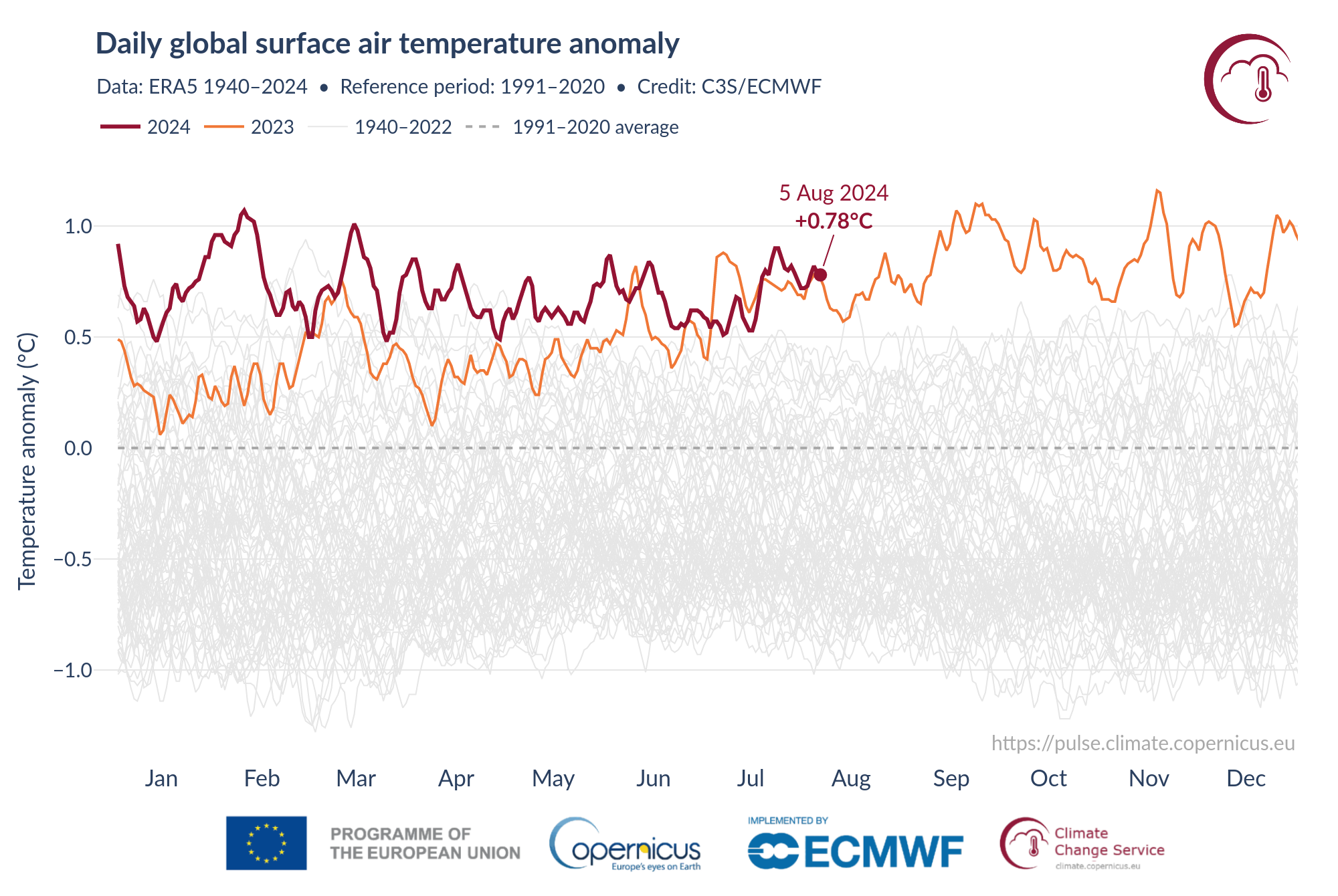
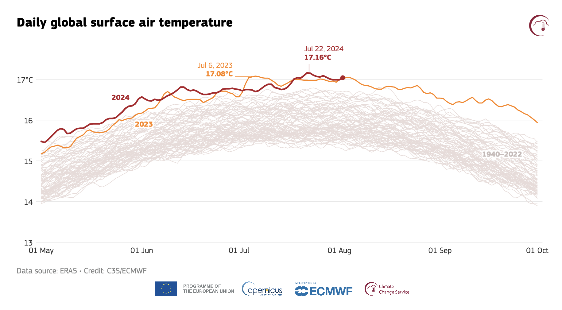
The past several years have been absolute scorchers, with 2023 being the warmest year ever recorded. And things did not slow down in 2024. As a result, we entered a stretch where every month set a new record as the warmest iteration of that month that we’ve ever recorded. Last month, that pattern stretched out for a full 12 months, as June of 2024 once again became the warmest June ever recorded. But, despite some exceptional temperatures in July, it fell just short of last July’s monthly temperature record, bringing the streak to a close.
Europe’s Copernicus system was first to announce that July of 2024 was ever so slightly cooler than July of 2023, missing out on setting a new record by just 0.04° C. So far, none of the other major climate trackers, such as Berkeley Earth or NASA GISS, have come out with data for July. These each have slightly different approaches to tracking temperatures, and, with a margin that small, it’s possible we’ll see one of them register last month as warmer or statistically indistinguishable.
How exceptional are the temperatures of the last few years? The EU averaged every July from 1991 to 2020—a period well after climate change had warmed the planet significantly—and July of 2024 was still 0.68° C above that average.
While it didn’t set a record, both the EU’s Copernicus climate service and NASA’s GISS found that it contained the warmest day ever recorded. In the EU’s case, they were the two hottest days recorded, as the temperatures on the 21st and 22nd were statistically indistinguishable, with only 0.01° C separating them. Late July and early August tend to be the warmest times of the year for surface air temperatures, so we’re likely past the point where any daily records will be set in 2024.
That’s all in terms of absolute temperatures. If you compare each day of the year only to instances of that day in the past, there have been far more anomalous days in the temperature record.
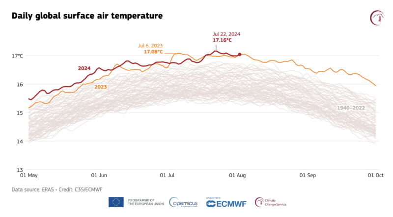
Enlarge/ In terms of anomalies over years past, both 2023 (orange) and 2024 (red) have been exceptionally warm.
That image also shows how exceptional the past year’s temperatures have been and makes it clear that 2024 is only falling out of record territory because the second half of 2023 was so exceptionally warm. It’s unlikely that 2024 will be quite as extreme, as the El Niño event that helped drive warming appears to have faded after peaking in December of 2023. NOAA’s latest forecast expects that the Pacific will remain in neutral for another month or two before starting to shift into cooler La Niña conditions before the year is out. (This is based on the August 8 ENSO forecast obtained here.)
In terms of anomalies, July also represents the first time in a year that a month had been less than 1.5° C above preindustrial temperatures (with preindustrial defined as the average over 1850–1900). Capping our modern temperatures at 1.5° C above preindustrial levels is recognized as a target that, while difficult to achieve, would help avoid some of the worst impacts we’ll see at 2° C of warming, and a number of countries have committed to that goal.
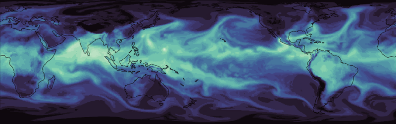
Enlarge/ Image of some of the atmospheric circulation seen during NeuralGCM runs.
Google
Right now, the world’s best weather forecast model is a General Circulation Model, or GCM, put together by the European Center for Medium-Range Weather Forecasts. A GCM is in part based on code that calculates the physics of various atmospheric processes that we understand well. For a lot of the rest, GCMs rely on what’s termed “parameterization,” which attempts to use empirically determined relationships to approximate what’s going on with processes where we don’t fully understand the physics.
Lately, GCMs have faced some competition from machine-learning techniques, which train AI systems to recognize patterns in meteorological data and use those to predict the conditions that will result over the next few days. Their forecasts, however, tend to get a bit vague after more than a few days and can’t deal with the sort of long-term factors that need to be considered when GCMs are used to study climate change.
On Monday, a team from Google’s AI group and the European Centre for Medium-Range Weather Forecasts are announcing NeuralGCM, a system that mixes physics-based atmospheric circulation with AI parameterization of other meteorological influences. Neural GCM is computationally efficient and performs very well in weather forecast benchmarks. Strikingly, it can also produce reasonable-looking output for runs that cover decades, potentially allowing it to address some climate-relevant questions. While it can’t handle a lot of what we use climate models for, there are some obvious routes for potential improvements.
Meet NeuralGCM
NeuralGCM is a two-part system. There’s what the researchers term a “dynamical core,” which handles the physics of large-scale atmospheric convection and takes into account basic physics like gravity and thermodynamics. Everything else is handled by the AI portion. “It’s everything that’s not in the equations of fluid dynamics,” said Google’s Stephan Hoyer. “So that means clouds, rainfall, solar radiation, drag across the surface of the Earth—also all the residual terms in the equations that happen below the grid scale of about roughly 100 kilometers or so.” It’s what you might call a monolithic AI. Rather than training individual modules that handle a single process, such as cloud formation, the AI portion is trained to deal with everything at once.
Critically, the whole system is trained concurrently rather than training the AI separately from the physics core. Initially, performance evaluations and updates to the neural network were performed at six-hour intervals since the system isn’t very stable until at least partially trained. Over time, those are stretched out to five days.
The result is a system that’s competitive with the best available for forecasts running out to 10 days, often exceeding the competition depending on the precise measure used (in addition to weather forecasting benchmarks, the researchers looked at features like tropical cyclones, atmospheric rivers, and the Intertropical Convergence Zone). On the longer forecasts, it tended to produce features that were less blurry than those made by pure AI forecasters, even though it was operating at a lower resolution than they were. This lower resolution means larger grid squares—the surface of the Earth is divided up into individual squares for computational purposes—than most other models, which cuts down significantly on its computing requirements.
Despite its success with weather, there were a couple of major caveats. One is that NeuralGCM tended to underestimate extreme events occurring in the tropics. The second is that it doesn’t actually model precipitation; instead, it calculates the balance between evaporation and precipitation.
But it also comes with some specific advantages over some other short-term forecast models, key among them being that it isn’t actually limited to running over the short term. The researchers let it run for up to two years, and it successfully reproduced a reasonable-looking seasonal cycle, including large-scale features of the atmospheric circulation. Other long-duration runs show that it can produce appropriate counts of tropical cyclones, which go on to follow trajectories that reflect patterns seen in the real world.
Because most things about Earth change so slowly, it’s difficult to imagine them being any different in the past. But Earth’s rotation has been slowing due to tidal interactions with the Moon, meaning that days were considerably shorter in the past. It’s easy to think that a 22-hour day wouldn’t be all that different, but that turns out not to be entirely true.
For example, some modeling has indicated that certain day lengths will be in resonance with other effects caused by the planet’s rotation, which can potentially offset the drag caused by the tides. Now, a new paper looks at how these resonances could affect the climate. The results suggest that it would shift rain to occurring in the morning and evening while leaving midday skies largely cloud-free. The resulting Earth would be considerably warmer.
On the Lamb
We’re all pretty familiar with the fact that the daytime Sun warms up the air. And those of us who remember high school chemistry will recall that a gas that is warmed will expand. So, it shouldn’t be a surprise to hear that the Earth’s atmosphere expands due to warming on its day side and contracts back again as it cools (these lag the daytime peak in sunlight). These differences provide something a bit like a handle that the gravitational pulls of the Sun and Moon can grab onto, exerting additional forces on the atmosphere. This complicated network of forces churns our atmosphere, helping shape the planet’s weather.
Two researchers, Russell Deitrick and Colin Goldblatt at Canada’s University of Victoria, were curious as to what would happen to these forces as the day length got shorter. Specifically, they were interested in a period where the day’s length would be at resonance with phenomena called Lamb waves.
Lamb waves aren’t specific to the atmosphere. Rather, they’re a specific manner in which a disturbance can travel through a medium, from vibrations in a solid to sound through the air.
Although various forces can create Lamb waves in the atmosphere, they’ll travel with a set of characteristic frequencies. One of those is roughly 10.5 to 11 hours. As you go back in time to shorter days, you’ll reach a point where the Earth’s day was a bit shorter than 22 hours, or twice the period of the Lamb waves. At this point, any disturbances in the atmosphere related to day length would have the ability to interact with the Lamb waves that were set off the day prior. This resonance could potentially strengthen the impact of any atmospheric phenomena related to day length.
Figuring out whether they do turned out to be a bit of a challenge. There are plenty of climate models to let researchers explore what’s going on in the modern atmosphere. But a lot of these have key features, like day length and solar output, hard coded into them. Others don’t let you do things like rearrange the Earth’s continents or change some atmospheric components.
The researchers did find a model that would allow them to change day length, solar intensity, and carbon dioxide concentrations to those present when Earth’s day length was 22 hours (which was likely to be in the pre-Cambrian). But it wasn’t able to reset the ozone concentrations, and ozone is also a greenhouse gas. So, they ran simulations without ozone, which are expected to be an under-estimate, and one where they elevated methane concentrations in order to mimic ozone’s greenhouse effect.
Enlarge/ A slice through an ice core showing bubbles of trapped air.
British Antarctic Survey
Did the massive scale of death in the Americas following colonial contact in the 1500s affect atmospheric CO2 levels? That’s a question scientists have debated over the last 30 years, ever since they noticed a sharp drop in CO2 around the year 1610 in air preserved in Antarctic ice.
That drop in atmospheric CO2 levels is the only significant decline in recent millennia, and scientists suggested that it was caused by reforestation in the Americas, which resulted from their depopulation via pandemics unleashed by early European contact. It is so distinct that it was proposed as a candidate for the marker of the beginning of a new geological epoch—the “Anthropocene.”
But the record from that ice core, taken at Law Dome in East Antarctica, shows that CO2 starts declining a bit late to match European contact, and it plummets over just 90 years, which is too drastic for feasible rates of vegetation regrowth. A different ice core, drilled in the West Antarctic, showed a more gradual decline starting earlier, but lacked the fine detail of the Law Dome ice.
Which one was right? Beyond the historical interest, it matters because it is a real-world, continent-scale test of reforestation’s effectiveness at removing CO2 from the atmosphere.
In a recent study, Amy King of the British Antarctic Survey and colleagues set out to test if the Law Dome data is a true reflection of atmospheric CO2 decline, using a new ice core drilled on the “Skytrain Ice Rise” in West Antarctica.
Precious tiny bubbles
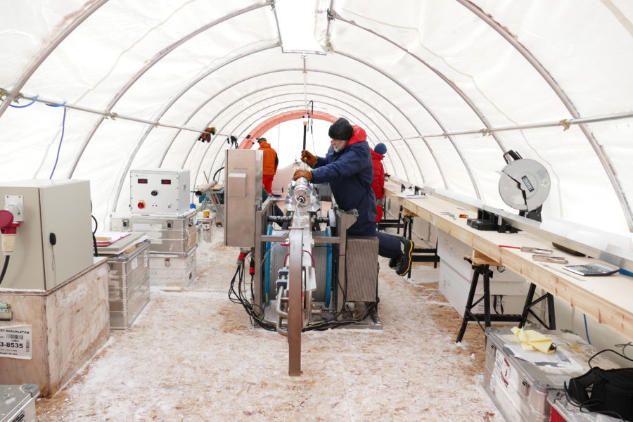
In 2018, scientists and engineers from the British Antarctic Survey and the University of Cambridge drilled the ice core, a cylinder of ice 651 meters long by 10 centimeters in diameter (2,136 feet by 4 inches), from the surface down to the bedrock. The ice contains bubbles of air that got trapped as snow fell, forming tiny capsules of past atmospheres.
The project’s main aim was to investigate ice from the time about 125,000 years ago when the climate was about as warm as it is today. But King and colleagues realized that the younger portion of ice could shed light on the 1610 CO2 decline.
“Given the resolution of what we could obtain with Skytrain Ice Rise, we predicted that, if the drop was real in the atmosphere as in Law Dome, we should see the drop in Skytrain, too,” said Thomas Bauska of the British Antarctic Survey, a co-author of the new study.
The ice core was cut into 80-centimeter (31-inch) lengths, put into insulated boxes, and shipped to the UK, all the while held at -20°C (-4°F) to prevent it from melting and releasing its precious cargo of air from millennia ago. “That’s one thing that keeps us up at night, especially as gas people,” said Bauska.
In the UK they took a series of samples across 31 depth intervals spanning the period from 1454 to 1688 CE: “We went in and sliced and diced our ice core as much as we could,” said Bauska. They sent the samples, still refrigerated, off to Oregon State University where the CO2 levels were measured.
The results didn’t show a sharp drop of CO2—instead, they showed a gentler CO2 decline of about 8 ppm over 157 years between 1516 and 1670 CE, matching the other West Antarctic ice core.
“We didn’t see the drop,” said Bauska, “so we had to say, OK, is our understanding of how smooth the records are accurate?”
A tent on the Antarctic ice where the core is cut into segments for shipping.
British Antarctic Survey
To test if the Skytrain ice record is too blurry to show a sharp 1610 drop, they analyzed the levels of methane in the ice. Because methane is much less soluble in water than CO2, they were able to melt continuously along the ice core to liberate the methane and get a more detailed graph of its concentration than was possible for CO2. If the atmospheric signal was blurred in Skytrain, it should have smoothed the methane record. But it didn’t.
“We didn’t see that really smoothed out methane record,” said Bauska, “which then told us the CO2 record couldn’t have been that smoothed.”
In other words, the gentler Skytrain CO2 signal is real, not an artifact.
Does this mean the sharp drop at 1610 in the Law Dome data is an artifact? It looks that way, but Bauska was cautious, saying, “the jury will still be out until we actually get either re-measurements of the Law Dome, or another ice core drilled with a similarly high accumulation.”
Freshwater is perhaps the world’s most essential resource, but climate change is enhancing its scarcity. An unexpected source may have the potential to provide some relief: offshore aquifers, giant undersea bodies of rock or sediment that hold and transport freshwater. But researchers don’t know how the water gets there, a question that needs to be resolved if we want to understand how to manage the water stored in them.
For decades, scientists have known about an aquifer off the US East Coast. It stretches from Martha’s Vineyard to New Jersey and holds almost as much water as two Lake Ontarios. Research presented at the American Geophysical Union conference in December attempted to explain where the water came from—a key step in finding out where other undersea aquifers lie hidden around the world.
As we discover and study more of them, offshore aquifers might become an unlikely resource for drinking water. Learning the water’s source can tell us if these freshwater reserves rebuild slowly over time or are a one-time-only emergency supply.
Reconstructing history
When ice sheets sat along the East Coast and the sea level was significantly lower than it is today, the coastline was around 100 kilometers further out to sea. Over time, freshwater filled small pockets in the open, sandy ground. Then, 10,000 years ago, the planet warmed, and sea levels rose, trapping the freshwater in the giant Continental Shelf Aquifer. But how that water came to be on the continental shelf in the first place is a mystery.
New Mexico Institute of Mining and Technology paleo-hydrogeologist Mark Person has been studying the aquifer since 1991. In the past three decades, he said, scientists’ understanding of the aquifer’s size, volume, and age has massively expanded. But they haven’t yet nailed down the water’s source, which could reveal where other submerged aquifers are hiding—if we learn the conditions that filled this one, we could look for other locations that had similar conditions.
“We can’t reenact Earth history,” Person said. Without the ability to conduct controlled experiments, scientists often resort to modeling to determine how geological structures formed millions of years ago. “It’s sort of like forensic workers looking at a crime scene,” he said.
Person developed three two-dimensional models of the offshore aquifer using seismic data and sediment and water samples from boreholes drilled onshore. Two models involved ice sheets melting; one did not.
Then, to corroborate the models, Person turned to isotopes—atoms with the same number of protons but different numbers of neutrons. Water mostly contains Oxygen-16, a lighter form of oxygen with two fewer neutrons than Oxygen-18.
Throughout the last million years, a cycle of planetary warming and cooling occurred every 100,000 years. During warming, the lighter 16O in the oceans evaporated into the atmosphere at a higher rate than the heavier 18O. During cooling, that lighter oxygen came down as snow, forming ice sheets with lower levels of 18O and leaving behind oceans with higher levels of 18O.
To determine if ice sheets played a role in forming the Continental Shelf Aquifer, Person explained, you have to look for water that is depleted in 18O—a sure sign that it came from ice sheets melting at their base. Person’s team used existing global isotope records from the shells of deep-ocean-dwelling animals near the aquifer. (The shells contain carbonate, an ion that includes oxygen pulled from the water).
Person then incorporated methods developed by a Columbia graduate student in 2019 that involve using electromagnetic imaging to finely map undersea aquifers. Since saltwater is more electrically conductive than freshwater, the boundaries between the two kinds of water are clear when electromagnetic pulses are sent through the seafloor: saltwater conducts the signal well, and freshwater doesn’t. What results looks sort of like a heat map, showing regions where fresh and saltwater are concentrated.
Person compared the electromagnetic and isotope data with his models to see which historical scenarios (ice or no ice) were statistically likely to form an aquifer that matched all the data. His results, which are in the review stage with the Geological Society of America Bulletin, suggest it’s very likely that ice sheets played a role in forming the aquifer.
“There’s a lot of uncertainty,” Person said, but “it’s the best thing we have going.”
Almost from the start, arguments about mitigating climate change have included an element of cost-benefit analysis: Would it cost more to move the world off fossil fuels than it would to simply try to adapt to a changing world? A strong consensus has built that the answer to the question is a clear no, capped off by a Nobel in Economics given to one of the people whose work was key to building that consensus.
While most academics may have considered the argument put to rest, it has enjoyed an extended life in the political sphere. Large unknowns remain about both the costs and benefits, which depend in part on the remaining uncertainties in climate science and in part on the assumptions baked into economic models.
In Wednesday’s edition of Nature, a small team of researchers analyzed how local economies have responded to the last 40 years of warming and projected those effects forward to 2050. They find that we’re already committed to warming that will see the growth of the global economy undercut by 20 percent. That places the cost of even a limited period of climate change at roughly six times the estimated price of putting the world on a path to limit the warming to 2° C.
Linking economics and climate
Many economic studies of climate change involve assumptions about the value of spending today to avoid the costs of a warmer climate in the future, as well as the details of those costs. But the people behind the new work, Maximilian Kotz, Anders Levermann, and Leonie Wenz decided to take an empirical approach. They obtained data about the economic performance of over 1,600 individual regions around the globe, going back 40 years. They then attempted to look for connections between that performance and climate events.
Previous research already identified a number of climate measures—average temperatures, daily temperature variability, total annual precipitation, the annual number of wet days, and extreme daily rainfall—that have all been linked to economic impacts. Some of these effects, like extreme rainfall, are likely to have immediate effects. Others on this list, like temperature variability, are likely to have a gradual impact that is only felt over time.
The researchers tested each factor for lagging effects, meaning an economic impact sometime after their onset. These suggested that temperature factors could have a lagging impact up to eight years after they changed, while precipitation changes were typically felt within four years of climate-driven changes. While this relationship might be in error for some of the economic changes in some regions, the inclusion of so many regions and a long time period should help limit the impact of those spurious correlations.
With the climate/economic relationship worked out, the researchers obtained climate projections from the Coupled Model Intercomparison Project (CMIP) project. With that in hand, they could look at future climates and estimate their economic costs.
Obviously, there are limits to how far into the future this process will work. The uncertainties of the climate models grow with time; the future economy starts looking a lot less like the present, and things like temperature extremes start to reach levels where past economic behavior no longer applies.
To deal with that, Kotz, Levermann, and Wenz performed a random sampling to determine the uncertainty in the system they developed. They look for the point where the uncertainties from the two most extreme emissions scenarios overlap. That occurs in 2049; after that, we can’t expect the past economic impacts of climate to apply.
Kotz, Levermann, and Wenz suggest that this is an indication of warming we’re already committed to, in part because the effect of past emissions hasn’t been felt in its entirety and partly because the global economy is a boat that turns slowly, so it will take time to implement significant changes in emissions. “Such a focus on the near term limits the large uncertainties about diverging future emission trajectories, the resulting long-term climate response and the validity of applying historically observed climate–economic relations over long timescales during which socio-technical conditions may change considerably,” they argue.
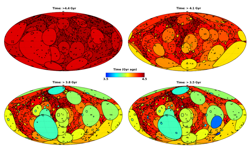
Enlarge/ Each panel shows the modeled effects of early Earth’s bombardment. Circles show the regions affected by each impact, with diameters corresponding to the final size of craters for impactors smaller than 100 kilometers in diameter. For larger impactors, the circle size corresponds to size of the region buried by impact-generated melt. Color coding indicates the timing of the impacts. The smallest impactors considered in this model have a diameter of 15 kilometers.
Simone Marchi, Southwest Research Institute
When it comes to space rocks slamming into Earth, two stand out. There’s the one that killed the dinosaurs 65 million years ago (goodbye T-rex, hello mammals!) and the one that formed Earth’s Moon. The asteroid that hurtled into the Yucatan peninsula and decimated the dinosaurs was a mere 10 kilometers in diameter. The impactor that formed the Moon, on the other hand, may have been about the size of Mars. But between the gigantic lunar-forming impact and the comparatively diminutive harbinger of dinosaurian death, Earth was certainly battered by other bodies.
When the Moon-forming impactor smashed into Earth, much of the world became a sea of melted rock called a magma ocean (if it wasn’t already melted). After this point, Earth had no more major additions of mass, said Simone Marchi, a planetary scientist at the Southwest Research Institute who creates computer models of the early Solar System and its planetary bodies, including Earth. “But you still have this debris flying about,” he said. This later phase of accretion may have lacked another lunar-scale impact, but likely featured large incoming asteroids. Predictions of the size and frequency distributions of this space flotsam indicate “that there has to be a substantial number of objects larger than, say, 1,000 kilometers in diameter,” Marchi said.
Unfortunately, there’s little obvious evidence in the rock record of these impacts before about 3.5 billion years ago. So scientists like Marchi can look to the Moon to estimate the number of objects that must have collided with Earth.
Armed with the size and number of impactors, Marchi and colleagues built a model that describes, as a function of time, the volume of melt this battering must have produced at the Earth’s surface. Magma oceans were in the past, but impactors greater than 100 kilometers in diameter still melted a lot of rock and must have drastically altered the early Earth.
Unlike smaller impacts, the volume of melt generated by objects of this size isn’t localized within a crater, according to models. Any crater exists only momentarily, as the rock is too fluid to maintain any sort of structure. Marchi compares this to tossing a stone into water. “There is a moment in time in which you have a cavity in the water, but then everything collapses and fills up because it’s a fluid.”
The melt volume is much larger than the amount of excavated rock, so Marchi can calculate just how much melt might have spilled out and coated parts of the Earth’s surface with each impact. The result is an astonishing map of melt volume. During the first billion years or so of Earth’s history, nearly the entire surface would have featured a veneer of impact melt at some point. Much of that history is gone because our active planet’s atmospheric, surface, and tectonic processes constantly modify much of the rock record.
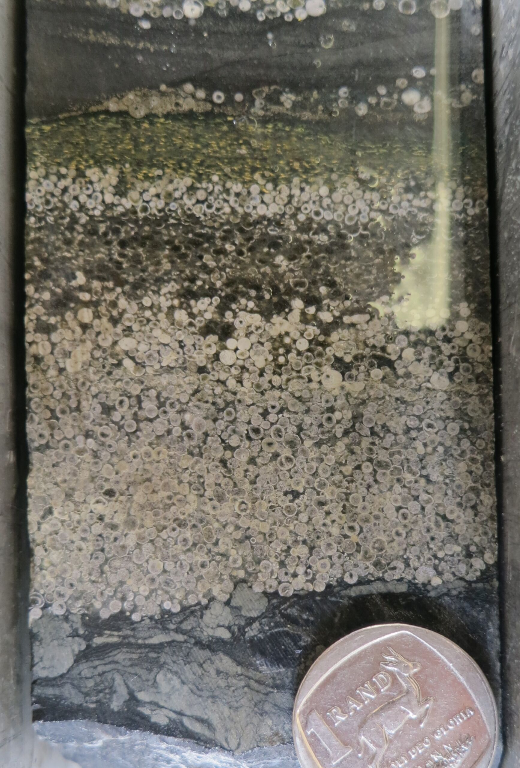
Balls of glass
Even between 3.5 and 2.5 billion years ago, the rock record is sparse. But two places, Australia and South Africa, preserve evidence of impacts in the form of spherules. These tiny glass balls form immediately after an impact that sends vaporized rock skyward. As the plume returns to Earth, small droplets begin to condense and rain down.


